Problem Set 1

Problem 1.1 Linear Transformation of a Random Variable

LOTUS

LOTUS (Law of the Unconscious Statistician) Theorem:

$$\begin{array}{rlrl}& \mathbb{E}\text{[}g(X)]=\sum \_xg(x)P(X=x)& \text{if descrete}& \\ & \mathbb{E}\text{[}g(X)]=\int \_{-\infty }^{\infty }g(x)f\_X(x),dx& \text{if continuous}& \end{array}$$

It’s all about sign cancelling

Transformation of probability density

the probability density function is defined as:

$$p\_Y(y)=\frac{d}{dy}F\_Y(y)=\frac{d}{dy}P(Y\le y)$$

given $y=g(x)$, to transform $P(Y\le y)$ to probability about $X$, slice $g$.

if $g$ is monotonically decrease in $\text{[}y\_1,y\_2]$

$$P(y\_1<Y\le y\_2)=P(g^{-1}(y\_2)<X\le g^{-1}(y\_1))=P(X\le g^{-1}(y\_1))-P(X\le g^{-1}(y\_2))$$

if $g$ is monotonically increase in $\text{[}y\_1,y\_2]$:

$$P(y\_1<Y\le y\_2)=P(X\le g^{-1}(y\_2))-P(X\le g^{-1}(y\_1))$$

take derivative of $x$, apply chain rule:

$$\frac{d}{dy}\int \_{-\infty }^{x}p\_x(t),dt=p\_x(x)\frac{dx}{dy}$$

and both cases generate the same expression:

$$\frac{d}{dx}P(y\_1<Y\le y\_2)=\frac{p\_x(x\_2)}{\left|g^{\prime }(y\_2)\right|}-\frac{p\_x(x\_1)}{\left|g^{\prime }(y\_1)\right|}$$

So for piecewise monotonic $g$:

$$p\_Y(y)=\frac{d}{dy}\sum \_kP(a\_k<Y\le b\_k)=p\_X(x)\left|\frac{dx}{dy}\right|$$

Proof of LOTUS

this leads to LOTUS:

the potential negative sign of $\frac{dy}{dx}$ also cancel with the potential flipping of integral limit caused by substituting variables in definite integral：

$$\mathbb{E}\text{[}y]=\int \_{-\infty }^{\infty }yp\_Y(y),dy=\int \_{-\infty }^{\infty }g(x)p\_X(x)\left|\frac{dx}{dy}\right|,d\left(\left|\frac{dy}{dx}\right|x\right)=\int \_{-\infty }^{\infty }g(x)p\_X(x),dx$$

Solutions

scalar case

Proof of $\mathbb{E}\text{[}ax+b]=a\mathbb{E}\text{[}x]+b$

definition of $\mathbb{E}\text{[}X]$

$$\mathbb{E}\text{[}X]=\int \_{-\infty }^{\infty }tf\_X(t),dt$$

applying LOTUS:

$$\begin{array}{rl}\mathbb{E}\text{[}ax]& =\int \_{-\infty }^{\infty }(ax)p(x),dx=a\int \_{-\infty }^{\infty }xp(x),dx=a\mathbb{E}\text{[}x]\\ \mathbb{E}\text{[}x+b]& =\int \_{-\infty }^{\infty }xp(x),dx+\int \_{-\infty }^{\infty }bp(x),dx=\mathbb{E}\text{[}x]+b\end{array}$$

Thus:

$$\begin{array}{rl}\mathbb{E}\text{[}ax+b]& =\mathbb{E}\text{[}(ax)+b]\\ & =\mathbb{E}\text{[}ax]+b\\ & =a\mathbb{E}\text{[}x]+b\end{array}$$

Proof of $\mathrm{var}(y)=a^2\mathrm{var}(x)$

Definition of $\mathrm{var}(X)$

\mathrm{var}(X) := \sigma^{2} :=\mathbb{E}\left\[ \left( X - \mu \right) ^{2} \right]

applying LOTUS, the direct consequence of the definition of $\mathrm{var}$ is:

$$\begin{array}{rl}\mathrm{var}(X)& =\mathbb{E}\text{[}{X}^2-2\mu X+{\mu }^2]\\ & =\mathbb{E}\text{[}{X}^2]-2{\mu }^2+{\mu }^2\\ & =\mathbb{E}\text{[}{X}^2]-{\mu }^2\end{array}$$

so:

\begin{align} \mathrm{var}(x+b) &= \mathbb{E}\left\[(x+b)^{2}\right] - \left(\mathbb{E}\[x+b]\right)^{2} \\ &= \mathbb{E}\[x^{2} + 2bx + b^{2}] - \left( \mu^{2} + 2b\mu + b^{2} \right) \\ & = \mathbb{E}\[x^{2}] - \mu^{2} = \mathrm{var}(x) \end{align} $$\begin{array}{rl}& \\ \mathrm{var}(ax)& =\mathbb{E}\text{[}(ax{)}^2]-{\left(\mathbb{E}\text{[}ax]\right)}^2\\ & =a^2\mathbb{E}\text{[}{x}^2]-a^2{\mu }^2=a^2\mathrm{var}(x)\end{array}$$

thus:

$$\mathrm{var}(ax+b)=\mathrm{var}(ax)=a^{2}var(x)$$

Vector case

Let’s say $x\in {\mathbb{R}}^d$, and $A\in {\mathbb{R}}^{m\times d},b\in {\mathbb{R}}^m,y=Ax+b$

Proof of $E\text{[}y]=AE\text{[}x]+b$:

Definition of expectation on a vector/matrix of random variables:

$$\mathbb{E}\text{[}X{]}_{i,j}=\mathbb{E}\text{[}{X}_{i,j}]$$

in the case of vector or matrix, addition is element-wise, so it’s easy to know:

$$\begin{array}{rl}\mathbb{E}\text{[}x+b]& =\mathbb{E}\text{[}x]+b\\ \mathbb{E}\text{[}X+B]& =\mathbb{E}\text{[}X]+B\\ \mathbb{E}\text{[}{x}^T]& =\mathbb{E}\text{[}x{]}^T\end{array}$$

When it comes to vector-multiplication, assume $a$ is a vector, and $x$ is a random variable, then the $i$-th element of vector $\mathbb{E}\text{[}ax]$ is:

$$\mathbb{E}\text{[}ax{]}_i=\mathbb{E}\text{[}{a}_{i}x]=a\_iE\text{[}x]$$

so $E\text{[}ax]=aE\text{[}x]$.

When it comes to matrix-multiplication, applying linearity of expectation in scalar space:

$$\begin{array}{rl}\mathbb{E}\text{[}Ax]& =\sum \_{k=1}^d\mathbb{E}\text{[}a\_kx\_k]\\ & =\sum \_{k=1}^{d}a\_k\mathbb{E}\text{[}x\_k]\\ & =A\mathbb{E}\text{[}x]\end{array}$$

thus:

$$\begin{array}{rl}\mathbb{E}\text{[}Ax+b]& =\mathbb{E}\text{[}Ax]+b\\ & =A\mathbb{E}\text{[}x]+b\end{array}$$

The definition of $\mathrm{cov}(x)$ is:

$$\mathrm{cov}(x{)}_{i,j}=\mathrm{cov}(x_i,x\_j)=\mathbb{E}\text{[}(x\_i-\mu \_i)(x\_j-\mu \_j)]$$ $$\begin{array}{rl}\mathrm{cov}(x{)}_{i,j}& =\mathbb{E}\text{[}{x}_{i}x\_j-\mu \_ix\_j-x\_i\mu \_j+\mu \_i\mu \_j]\\ & =\mathbb{E}\text{[}x\_ix\_j]-\mu \_i\mu \_j\end{array}$$

This match the outer product rule:

$$\mathrm{cov}(x)=\mathbb{E}\text{[}x{x}^T]-\mu {\mu }^T$$

applying the rule $(x+y)(x+y{)}^T=x{x}^T+y{x}^T+x{y}^T+y{y}^T$：

$$\begin{array}{rl}\mathrm{cov}(x+b)& =\mathbb{E}\text{[}(X+b)(X+b{)}^T]-(\mu +b)(\mu +b{)}^T\\ & =\mathbb{E}\text{[}x{x}^T+b{x}^T+x{b}^T+b{b}^T]-(\mu {\mu }^T+b{\mu }^T+\mu b^T+b{b}^T)\\ & =\mathbb{E}\text{[}x{x}^T]-\mu {\mu }^T=\mathrm{cov}(x)\end{array}$$ $$\mathbb{E}\text{[}{x}^T{A}^T]=\sum \_{k=1}^{d}E\text{[}x\_k]a\_k^T=\mathbb{E}\text{[}x{]}^T{A}^T$$

applying the rule $(Ax)(Ax{)}^T=Ax{x}^T{A}^T$

$$\begin{array}{rl}\mathrm{cov}(Ax)& =\mathbb{E}\text{[}(Ax)(Ax{)}^T]-\mathbb{E}\text{[}Ax]E\text{[}Ax{]}^T\\ & =\mathbb{E}\text{[}Ax{x}^T{A}^T]-(A\mathbb{E}\text{[}x])(A\mathbb{E}\text{[}x]{)}^T\\ & =A\mathbb{E}\text{[}x{x}^T]A^T-A\mathbb{E}\text{[}x]\mathbb{E}\text{[}x{]}^T{A}^T\\ & =A\left(\mathbb{E}\text{[}x{x}^T]-\mathbb{E}\text{[}x]\mathbb{E}\text{[}x{]}^T\right)A^T\\ & =A\mathrm{cov}{A}^T\end{array}$$

with the results above, we have:

$$\mathrm{cov}(Ax+b)=A\mathrm{cov}(x)A^T$$

Problem 1.2 Properties of Independence

multivariate version of LOTUS (continuous case):

$$\mathbb{E}\text{[}g(x\_1,\dots ,x\_n)]=\int \_{-\infty }^{\infty }g(x\_1,\dots ,x\_n)f(x\_1,\dots ,x\_n),dx\_1\dots x\_n$$

independency implies the joint probability density is the product of the marginal probability density:

$$\begin{array}{rl}X\perp Y& ⟹P(X\le x,Y\le y)=P(X\le x)P(X\le y)\\ & ⟹f\_X,Y(x,y)=f\_X(x)f\_Y(y)\end{array}$$

By applying both LOTUS:

$$\begin{array}{rl}\mathbb{E}\text{[}xy]& =\int \_{-\infty }^{\infty }\int \_{-\infty }^{\infty }(xy)f(x,y),dxdy\\ & =\int \_{-\infty }^{\infty }\int \_{-\infty }^{\infty }xyf(x)f(y),dx,dy\\ & =\int \_{-\infty }^{\infty }xf(x),dx\int \_{-\infty }^{\infty }yf(y),dy\\ & =\mathbb{E}\text{[}x]\mathbb{E}\text{[}y]\end{array}$$

so for $\mathrm{cov}(x,y)$, it will be zero if $x$ and $y$ are independent:

$$\mathrm{cov}(\mathrm{x},\mathrm{y})=\mathbb{E}\text{[}xy]-\mathbb{E}\text{[}x]\mathbb{E}\text{[}y]=0$$

Problem 1.3 Uncorrelated vs Independence

Relationship uncorrelated: \left{ (x,y) | \mathrm{cov}(x,y)=0 \right} uncorrelated $/⟹$ independence, independence $⟹$ uncorrelated

$x$ and $y$ are uncorrelated:

\begin{align} \mu\_{x} &= \sum\_{x} \frac{1}{4} x = \frac{1}{4} (1 + 0 + -1 + 0) = 0 \\ \mu\_{y} & = \sum\_{y} \frac{1}{4} y = \frac{1}{4}(0 + 1 + 0 + -1) = 0 \\ \mathrm{cov}(x, y) &= \sum\_{x} \sum\_{y} \frac{1}{4} (x - \mu\_{x}) (y - \mu\_{y}) \\ &=\frac{1}{4} \sum\_{x} \sum\_{y} xy \\ &= \frac{1}{4} \left\[ (1\times 0) + (0 \times 1) + (-1 \times 1) + (0 \times -1) \right] \\ & = 0 \end{align}

marginal distribution:

p(x,y)	-1	0	1	p(x)
-1		1/4		1/4
0	1/4		1/4	1/2
1		1/4		1/4
p(y)	1/4	1/2	1/4	1

it’s apparently that $p(x=0,y=0)=0$, but $p(x=0)p(y=0)=\frac{1}{2}$, $p(x,y)\ne p(x)p(y)$ at $(0,0)$, so $x$ and $y$ are not independent.

definition of the conditional expectation:

$$\mathbb{E}\text{[}x|y]=\int \_Xxf(x|y)dx$$

by law of total expectation:

$$\begin{array}{rl}\mathbb{E}\text{[}XY]& =\mathbb{E}\text{[}\mathbb{E}\text{[}XY|Y]]\\ & =\mathbb{E}\text{[}Y\mathbb{E}\text{[}X|Y]]\\ & =\mathbb{E}\text{[}Y\mathbb{E}\text{[}X]]\\ & =\mathbb{E}\text{[}X]\mathbb{E}\text{[}Y]\end{array}$$

$\mathbb{E}\text{[}XY]=\mathbb{E}\text{[}X]\text{[}\mathbb{E}\text{[}Y]⟹\mathrm{cov}(x,y)=0$ is proven above, so $x$ and $y$ are uncorrelated.

Law of Total Expectation

Or called Iterated Expectation: take expectation on conditioned variables and then conditions generate the expectation on the joint distribution.

$$\begin{array}{rl}\mathbb{E}\text{[}\mathbb{E}\text{[}g(x,y)|y]]& =\int \_Y\mathbb{E}\text{[}g(x,y)|y]f(y)dy\\ & =\int \_Y\int \_Xg(x,y)\frac{f(x,y)}{f(y)}dxf(y)dy\\ & =\int \_Y\int \_Xg(x,y)f(x,y),dxdy=\mathbb{E}\text{[}g(x,y)]\end{array}$$

Problem 1.4 Sum of Random Variables

For any $x,y$:

$$\begin{array}{rl}\mathbb{E}\text{[}x+y]& =\int \_X\int \_Y(x+y)f(x,y)dxdy\\ & =\int \_X\int \_Yxf(x,y)dxdy+\int \_X\int \_Yyf(x,y)dxdy\\ & =\int \_Xx\left(\int \_Yf(x,y)dy\right)dx+\int \_Yy\left(\int \_Xxf(x,y)dx\right)dy\\ & =\int \_Xxf\_x(x)dx+\int \_Yyf\_y(y)dy\\ & =\mathbb{E}\text{[}x]+\mathbb{E}\text{[}y]\end{array}$$

when $x$ and $y$ are independent, we have $\mathbb{E}\text{[}xy]=\mathbb{E}\text{[}x]\mathbb{E}\text{[}y]$, so:

\begin{align} \mathrm{var}(x + y) &= \mathbb{E}\left\[ \left( x + y - \mu\_{xy} \right) ^2 \right] \\ &= \mathbb{E}\[x^2 + y^2 + 2xy -2\mu\_{xy}(x+y)+ \mu\_{xy}^{2}] \\ &= \mathbb{E}\[x^{2}] + \mathbb{E}\[y^{2}] + 2\mathbb{E}\[xy] - 2\mu\_{xy} (\mathbb{E}\[x] + \mathbb{E}\[y]) + \mu\_{xy}^{2} \\ &= \mathbb{E}\[x^{2}] + \mathbb{E}\[y^{2}] + 2\mathbb{E}\[x]\mathbb{E}\[y] - 2(\mathbb{E}\[x] + \mathbb{E}\[y] )^{2} + (\mathbb{E}\[x] + \mathbb{E}\[y])^{2} \\ &= \mathbb{E}\[x^{2}] + \mathbb{E}\[y^{2}] - \mathbb{E}\[x]^{2}-\mathbb{E}\[y]^{2} \\ &= \mathrm{var}(x) + \mathrm{var(y)} \\ \end{align}

Problem 1.5 Expectation of an Indicator Variable

$$\begin{array}{rl}\mathbb{E}\text{[}x]& =0p(x=0)+1p(x=1)=p(x=1)\\ \mathrm{var}(x)& =(0-p(x=1){)}^{2}p(x=0)+(1-p(x=1){)}^{2}p(x=1)\\ & =p(x=1{)}^{2}p(x=0)+p(x=0{)}^{2}p(x=1)\\ & =p(x=0)p(x=1)\end{array}$$

Problem 1.6 Multivariate Gaussian

Quadratic Form 二次型

$$x^{T}Ax=\sum \_i\sum \_ja\_i,jx\_ix\_j$$

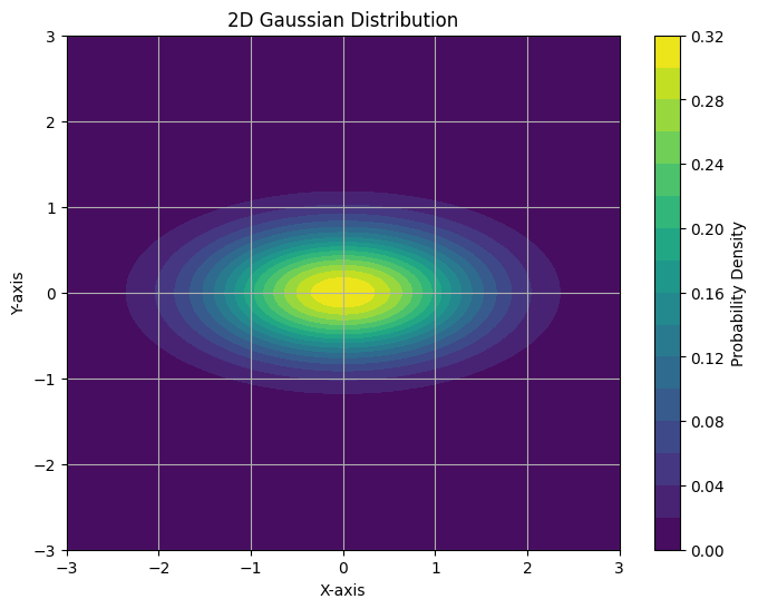
Multivariate Gaussian: a probability density over real vectors (join probability)

$$p(x)=\mathcal{N}(x|\mu ,\Sigma )=\frac{1}{(2\pi {)}^{d/2}|\sigma {|}^{1/2}}{e}^{-1/2||x-\mu ||\_{\Sigma }^2}$$

With a diagonal convariance matrix:

$$\Sigma =\left[\begin{array}{ccc}\sigma \_1^2& \dots & 0\\ ⋮& \ddots & ⋮\\ 0& \dots & \sigma \_d^2\end{array}\right]$$

The Mahalanobis distance would be:

$$\begin{array}{rl}||x-\mu |{|}_{\Sigma }^2& =\sum _{i=1}^d\frac{(x\_i-\mu \_i{)}^2}{\sigma \_i^2}\end{array}$$

The determinant of $\Sigma$ would be:

$$|\Sigma |=\prod \_{i=1}^d\sigma \_i^2$$

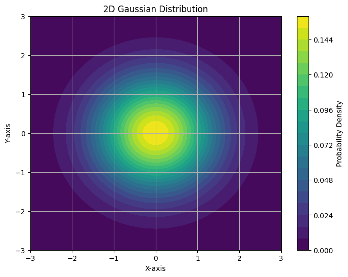
So the density becomes the product of univariate gaussian, indicating that a diagonal covariant matrix make sure the variables are independent:

$$\begin{array}{rl}\mathcal{N}(x|\mu ,\Sigma )& =\frac{1}{(2\pi {)}^{d/2}\prod \_{i=1}^d\sigma \_i}\exp \left(-\frac{1}{2}\sum \_{i=1}^d\frac{(x\_i-\mu \_i{)}^2}{\sigma \_i^2}\right)\\ & =\prod \_{i=1}^d\frac{1}{(2\pi {)}^{1/2}\sigma \_i}\exp \left(-\frac{1}{2}\frac{(x\_i-\mu \_i{)}^2}{\sigma \_i^2}\right)\\ & =\prod \_{i=1}^d\mathcal{N}(x\_i|\mu \_i,\sigma \_i^2)\end{array}$$

with $\mu =\left[\begin{array}{c}00\end{array}\right],\Sigma =\left[\begin{array}{ccc}1& 00& 0.25\end{array}\right]$, the gaussian is squeezed in y dimension.

with $\mu =\left[\begin{array}{c}00\end{array}\right],\Sigma =\left[\begin{array}{ccc}1& 00& 1\end{array}\right]$, all components are i.i.d.

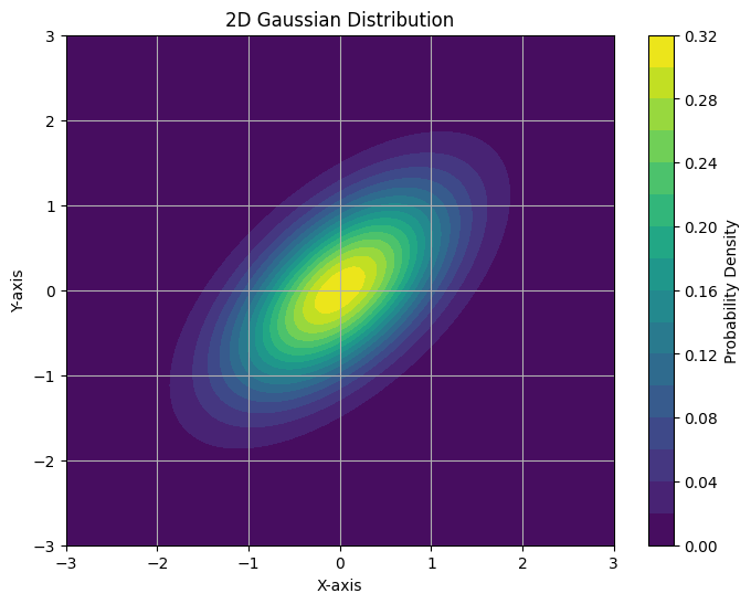
eigen-decompose

$$\Sigma =V\Lambda V^T$$

let $y=V^T(x-\mu )$ Mahalanobis distance could be:

$$\begin{array}{rl}||x-\mu |{|}_{\Sigma }^2& =(x-\mu {)}^{T}V\Lambda V^T(x-\mu )\\ & =\left((x-\mu {)}^{T}V\right)\Lambda \left(V^T(x-\mu )\right)\\ & =y^T\Lambda y\\ & =||y|{|}_{\Lambda }^2\end{array}$$

$\mu$: centering $x$ $V$: rotate and scale $x$, so they are independent and normalized.

Eigenvalue and Eigenvector: $Av=\lambda v$, Since $0$ is a solution for $(A-I\lambda )v=0$, to get additional values, its determinant should be zero. Apply this idea to $\Sigma$:

$$\begin{array}{r}\det \left(\Sigma -I\lambda \right)=0\\ (0.625-\lambda {)}^2=0.375^2\\ \lambda \_1=0.250,\lambda \_2=1.000\\ v\_1=\text{[}1,-1],v\_2=\text{[}1,1]\end{array}$$

Eigenvector define the direction, and small eigenvalue center the distribution, while large eigenvalue sparse the distribution (more covariance).

Problem 1.7 Product of Gaussian Distributions

\begin{align} \mathcal{N} (x | \mu\_{1}, \sigma\_{1}^{2}) &\mathcal{N} (x | \mu\_{2}, \sigma\_{2}^{2})\\ \= & \frac{1}{\sqrt{2\pi} \sigma\_{1}^{2}} \frac{1}{\sqrt{ 2\pi } \sigma\_{2}^{2}}\exp\left( -\frac{1}{2} \left( \frac{(x-\mu\_{1})^{2}}{\sigma\_{1}^{2}} + \frac{(x-\mu\_{2})^{2}}{\sigma\_{2}^{2}} \right) \right) \\ \= & \frac{1}{\sqrt{2\pi} \sigma\_{1}^{2}} \frac{1}{\sqrt{ 2\pi } \sigma\_{2}^{2}}\exp\left( -\frac{1}{2} \frac{\left( (\sigma\_{1}^{2} + \sigma\_{2}^{2})x^{2}-2(\mu\_{1}\sigma\_{2}^{2} + \mu\_{2}\sigma\_{1}^{2})x + (\mu\_{1}^{2}\sigma\_{2}^{2}+\mu\_{2}^{2}\sigma\_{1}^{2})\right)}{\sigma\_{1}^{2}\sigma\_{2}^{2}} \right) \\ \end{align}

$a{x}^2-2bx=a{\left(x-\frac{b}{a}\right)}^2-\frac{b^2}{a^2}$

transform:

$$(\sigma \_1^2+\sigma \_2^2){\left(x-\frac{\mu \sigma \_2^2+\mu \_2\sigma \_1^2}{\sigma \_1^2+\sigma \_2^2}\right)}^2-{\left(\frac{\mu \_1\sigma \_2^2+\mu \_2\sigma \_1^2}{\sigma \_1^2+\sigma \_2^2}\right)}^2$$

A Gaussian distribution can be identified:

$$\begin{array}{rl}\sigma \_3^2& =\frac{\sigma \_1^2\sigma \_2^2}{\sigma \_1^2+\sigma \_2^2}=\frac{1}{\sigma \_1^{-2}+\sigma \_2^{-2}}\\ \mu \_3& =\frac{\mu \_1\sigma \_2^2+\mu \_2\sigma \_1^2}{\sigma \_1^2+\sigma \_2^2}=\sigma \_3^2(\mu \_1\sigma \_2^{-2}+\mu \_2\sigma \_1^{-2})\end{array}$$

Now process the rest of the expression

the remaining part of exponent part of $\exp$ is $-\frac{1}{2}$ times:

\begin{align} &\frac{(\mu\_{1}^{2}\sigma\_{2}^{2}+\mu\_{2}^{2}\sigma\_{1}^{2})}{\sigma\_{1}^{2}\sigma\_{2}^{2}} - \frac{\left(\frac{\mu\_{1}\sigma\_{2}^{2}+\mu\_{2}\sigma\_{1}^{2}}{\sigma\_{1}^{2}+\sigma\_{2}^{2}}\right)^{2}}{\sigma\_{1}^{2}\sigma\_{2}^{2}} \\ \=& \frac{(\mu\_{1}^{2}\sigma\_{2}^{2}+\mu\_{2}^{2}\sigma\_{1}^{2})(\sigma\_{1}^{2}+\sigma\_{2}^{2})}{\sigma\_{1}^{2}\sigma\_{2}^{2}(\sigma\_{1}^{2}+\sigma\_{2}^{2})} - \frac{\mu\_{1}^{2}\sigma\_{2}^{4}+\mu\_{2}^{2}\sigma\_{1}^{4} + 2\mu\_{1}\mu\_{2}\sigma\_{1}^{2}\sigma\_{2}^{2}}{\sigma\_{1}^{2}\sigma\_{2}^{2}(\sigma\_{1}^{2}+\sigma\_{2}^{2})} \\ \=& \frac{\left(\mu\_{1}^{2}+\mu\_{2}^{2}\sigma\_{1}^{2}\sigma\_{2}^{-2}+\mu\_{1}^{2}\sigma\_{1}^{-2}\sigma\_{2}^{2} + \mu\_{2}^{2} \right) - \left(\mu\_{1}^{2}\sigma\_{1}^{-2}\sigma\_{2}^{2} + \mu\_{2}^{2}\sigma\_{1}^{2}\sigma\_{2}^{-2} + 2\mu\_{1}\mu\_{2} \right)}{\sigma\_{1}^{2}+\sigma\_{2}^{2}} \\ \=& \frac{(\mu\_{1} - \mu\_{2})^{2}}{\sigma\_{1}^{2}+\sigma\_{2}^{2}} \end{align}

This could also be treated as an fixed value Gaussian:

$$\frac{1}{\sqrt{2\pi (\sigma \_1^2+\sigma \_2^2)}}\exp \left(-\frac{1}{2}\frac{(\mu \_1-\mu \_2{)}^2}{\sigma \_1^2+\sigma \_2^2}\right)=\mathcal{N}(\mu \_1|\mu \_2,\sigma \_1^2+\sigma \_2^2)=Z$$

And the Remaining factor is:

\begin{align} &\sqrt{ 2\pi(\sigma\_{1}^{2} + \sigma\_{2}^{2}) } \frac{1}{\sqrt{ 2\pi } \sigma\_{1}^{2}} \frac{1}{\sqrt{ 2\pi}\sigma\_{2}^{2}} \\ \=& \frac{\sigma\_{1}^{-2}+ \sigma\_{2}^{-2}}{\sqrt{ 2\pi }} \\ \=& \frac{1}{\sqrt{ 2\pi }\sigma\_{3}^{2}} \end{align}

which match the form of Gaussian together with the exponential part. So the overall distribution expression is:

$$\mathcal{N}(x|\mu \_1,\sigma \_1^2)\mathcal{N}(x|\mu \_2,\sigma \_2^2)=Z\mathcal{N}(x|\mu \_3,\sigma \_3^2)$$

The resulting scaled Gaussian means this could not hold unless the scaling factor is 1

Problem 1.8 Product of Multivariate Gaussian Distributions

\begin{align} & \mathcal{N}(x | a, A) \mathcal{N}(x | b, B) \\ \=& \frac{1}{(2\pi)^{d/2}|A|^{1/2}}\exp\left( -\frac{1}{2}||x-a||_{A}^{2} \right) \frac{1}{(2\pi)^{d/2}|B|^{1/2}}\exp\left( -\frac{1}{2}||x-b||_{B}^{2} \right) \\ \=& \frac{1}{(2\pi)^{d}|A|^{1/2}|B|^{1/2}} \exp\left( -\frac{1}{2} \left( (x-a)^TA^{-1}(x-a) + (x-b)^T B^{-1} (x-b) \right) \right) \\ \end{align}

expand the exponent term, and then complete the square:

\begin{align} \&x^T(A^{-1}+B^{-1})x-2x^T(A^{-1}a +B^{-1}b) + a^TA^{-1}a + b^TB^{-1}b \\ \=& (x - c)^T(A^{-1} + B^{-1}) (x - c) + e \\ \\ C=&(A^{-1}+B^{-1})^{-1} \\ c=& C(A^{-1}a + B^{-1}b) \\ e=& (a^T A^{-1} a + b^TB^{-1}b) - (A^{-1}a + B^{-1}b)^T(A^{-1}+B^{-1})^{-1}(A^{-1}a + B^{-1}b) \\ \=& \dots& \end{align}

so the Gaussian part of the product is:

$$\frac{1}{(2\pi {)}^{d/2}|C{|}^{1/2}}\exp \left(-\frac{1}{2}\left((x-c{)}^T(A^{-1}+B^{-1})(x-c)\right)\right)$$

leaving the coefficient as:

$$\begin{array}{rl}& \frac{|A^{-1}+B^{-1}{|}^{1/2}}{(2\pi {)}^{2/d}|A{|}^{1/2}|B{|}^{1/2}}\end{array}$$

to figure out $e$, apply Woodbury matrix identity to simplify the nested inverse. Simply applying Woodbury Identity introduce two terms, so we make further transformation:

\begin{align} (A^{-1} + B^{-1})^{-1} &= A - A(B + A)^{-1}A \\ &= A(B+A)^{-1} \left\[ (B+A) - A \right] \\ & = A(A+B)^{-1}B \end{align}

so the last term of e should be:

\begin{align} & (a^TA^{-1} + b^{T}B^{-1})(A(A+B)^{-1}B)(A^{-1}a + B^{-1}b) \\ \=& (a^{T} + b^{T}B^{-1}A)(A+B)^{-1} (BA^{-1}a + b) \\ \= & a^{T}(A+B)^{-1}BA^{-1}a + b^{T}B^{-1}A(A+B)^{-1}BA^{-1}a + a^{T}(A+B)^{-1}b + b^{T}B^{-1}A(A+B)^{-1}b \\ \end{align}

Combining the two terms in $e$ would have:

\begin{align} & \left(a^{T}A^{-1}a - a^{T}(A+B)^{-1}BA^{-1}a \right) \\ \=& a^{T} \left( I - (A+B)^{-1}B \right) A^{-1}a \\ \=& a^{T}(A+B)^{-1}a \end{align}

also:

\begin{align} & (b^{T}B^{-1}b - b^{T}B^{-1}A(A+B)^{-1}b) \\ \=& b^{T}B^{-1}(I - A(A+B)^{-1})b \\ \=& b^{T}(A+B)^{-1}b \end{align}

observe the second term, we apply Exchange Identity $A(A+B{)}^{-1}B=B(A+B{)}^{-1}A$ here:

$$b^T{B}^{-1}A(A+B{)}^{-1}B{A}^{-1}a=b^T(A+B{)}^{-1}a$$

and since $(A+B{)}^{-1}$ is symmetric, so $b^T(A+B{)}^{-1}a=a^T(A+B{)}^{-1}b$

$$\begin{array}{rl}e& =a^T(A+B{)}^{-1}a-2a^T(A+B{)}^{-1}b+b^T(A+B{)}^{-1}b\\ & =(a-b{)}^T(A+B{)}^{-1}(a-b)\end{array}$$

and the coefficient is:

\begin{align} & \frac{|A^{-1}+B^{-1}|^{1/2}}{(2\pi)^{d/2} |A|^{1/2}|B|^{1/2}} \\ \=& \frac{|A(A+B)^{-1}B|^{1/2}}{(2\pi)^{d/2} |A|^{1/2}|B|^{1/2}} \\ \=& \frac{1}{(2\pi)^{d/2}|A+B|^{1/2}} \end{align}

This transformation procedure use a lot rules of Determinant

The coefficient and the redundant exponential term also form a fixed-value Gaussian:

$$Z=\mathcal{N}(a|b,A+B)$$

So the product of multivariable Gaussian is:

$$\mathcal{N}(x|a,A)\mathcal{N}(y|b,B)=Z\mathcal{N}(x|c,C)$$

Woodbury Matrix Identity

Inverting after low rank modification with low cost

$${\left(A+UCV\right)}^{-1}=A^{-1}-A^{-1}U(C^{-1}+V{A}^{-1}U{)}^{-1}V{A}^{-1}$$

Motivation: if you’ve inverted a large matrix $A$, inverting it after added a low-rank update $UCV$ should not have to start from scratch

$$A+UCV$$

• $C$: the core update, $k\times k$
• $U,V$: bring the update $C$ into the space of $A$, $n\times k,k\times n$

How to construct the invert

• subtract the correction: adding something to the original matrix usually “shrink” the inverse \begin{align} &(A+UCV)(A^{-1} - \mathrm{Correction})\\ \=& (I + UCVA^{-1}) - (A+UCV)(\mathrm{Correction}) \\ \=& I + UCVA^{-1} - UC(C^{-1}U^{-1}A + V)(\mathrm{Correction}) \end{align}

To cancel the last to terms, we can build correction with a sandwich structure to match the terms of $UCV{A}^{-1}$:

1. there is a $V{A}^{-1}$ in the back
2. we don’t want to invert $U^{-1}$, even it’s invertible, so there should be a $A^{-1}U$ in the form
3. let’s call the remaining part $R$ So the Correction term should have the form: $$\mathrm{Correction}=AURV{A}^{-1}$$ so we have the last term as: $$UC(C^{-1}+VAU)RV{A}^{-1}$$ The only unknown matrix here is $R$, compare with $UCV{A}^{-1}$, the only difference is the last term has a $(C^{-1}+VAU)R$ inside, making this $I$ so we are able to cancel these two terms:

$$R=(C^{-1}+VAU{)}^{-1}$$

So the correction term should be

$$A^{-1}U(C^{-1}+VAU{)}^{-1}V{A}^{-1}$$

the inverse should belike:

$$A^{-1}-A^{-1}U(C^{-1}+VAU{)}^{-1}V{A}^{-1}$$

Notice that we assume $U$ is invertible, which does not always hold. But surprisingly this form also hold when $U$ is not invertible. It can be verified by the same process above.

Problem 1.9 Correlation between Gaussian Distributions

Warning

Do not mix the concept of Correlation and Covariance

correlation between distribution is defined as:

$$\int f\_X(x)f\_Y(x)dx$$

Using problem 1.8, The correlation between two Gaussian distributions is:

\begin{align} & \int \mathcal{N}(x|a,A)\mathcal{N}(x|b,B) dx \\ \=& \int \mathcal{N}(a|b, A + B) \mathcal{N} (x|c, C) dx \\ \=& \mathcal{N}(a|b, A+ B) \end{align}

Problem 1.10 Completing the square

$$\begin{array}{rl}f(x)& =(x-d{)}^{T}A(x-d)+e\\ & =(x^T-d^T)A(x-d)+e\\ & =x^{T}Ax-d^{T}Ax-x^{T}Ad+d^{T}Ad+e\\ & =x^{T}Ax-2x^{T}Ad+d^{T}Ad+e\\ & =x^{T}Ax-2x^{T}b+c\\ & \\ d& =A^{-1}b\\ e& =c-d^{T}Ad=c-b^T(A^{-1}{)}^{T}b\end{array}$$

Problems 1.11 Eigenvalues

trace is defined as the sum of the diagonal

$$\mathrm{Tr}(A)=\sum \_{i=1}^{n}A\_ii$$

eigenvalues are roots of the characteristic function:

$$p(\lambda )=\det (A-\lambda I)=\prod \_{i=1}^n(\lambda \_i-\lambda )$$

the latter equivalence is guarantee by Identity Theorem for Polynomials

let $\lambda =0$, then:

$$p(0)=\det (A)=\prod \_{i=1}^n\lambda \_i$$

Problems 1.12 Eigenvalues of an inverse matrix

Problems 1.13 Positive Definiteness